I cannot do but drool at the eleganceof this #julialang code, once you get the hang of how to do things (i.e. thinking the other way round).

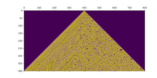
Here's a short snippet that produces Wolfram's one-dimensional cellular automatons. Generation 0 is easily created, next-generation is a simple mapping of one generation vector mapping from n to n+1, and Wolfram's elementary cellular automaton number has been converted to a Hash-Mapped value in 3-dimensional dual space {0,1}[3]. Sheer elegance.

One can also see that mapping g: n -> n+1 contains an "observer problem". One must make a decision what to do with the outermost pixels for which no three predecessors are defined. In the case of starting from one center value, that's not a problem, as long as the width is twice the height. But if you redesign the automaton to run from a random starting vector, a decision has to be made what to do with the corner pixels:

• Assume overflow-0
• Assume overflow-1
• Assume the value of the preceding row

So within any rectangle that does not contain the original starting point, the automaton cannot be run without the conditions of observation (section rectangle) influencing the simulation. Classical observer problem.

using PyPlot

function gen0(n)
    [zeros(Int, div(n,2)); 1; zeros(Int,div(n,2))]
end

function genN(a, f)
    [0; [f[a[i-1]+1, a[i]+1, a[i+1]+1] for i in 2:length(a)-1] ; 0]
end

function mkruleset(r)
    [(r & 2^(4*a + 2b + c) > 0 ? 1 : 0)  for a in 0:1, b in 0:1, c in 0:1 ]
end

function crecurse(x0, g, r, N, cond)
    # init vector, generation func, ruleset, max steps, exit condition
    n = 0

    X = [x0]
    while n < N && !cond(X[end])
        n += 1
        X = [X[:]; [g(X[end], r)]]
    end

    X
end

rule = 30
lines = 400
width = 800

M = crecurse(gen0(width), genN, mkruleset(rule), lines, iszero)
matshow(M)